神经网络学习笔记(12) – 生成对抗网络
生成对抗网络Generative Adversarial Networks,简称(GANs)。其思想是用两个神经网络互相对抗,以生成一些“真实”的图像或视频。它的应用包括:AI艺术,人造图像,从2维图像生成3维图像,以及传统的分类、回归问题等。
两个对抗网络的分别为:生成网络(Generative network)和判别网络(Discriminative network)。
它的架构如下: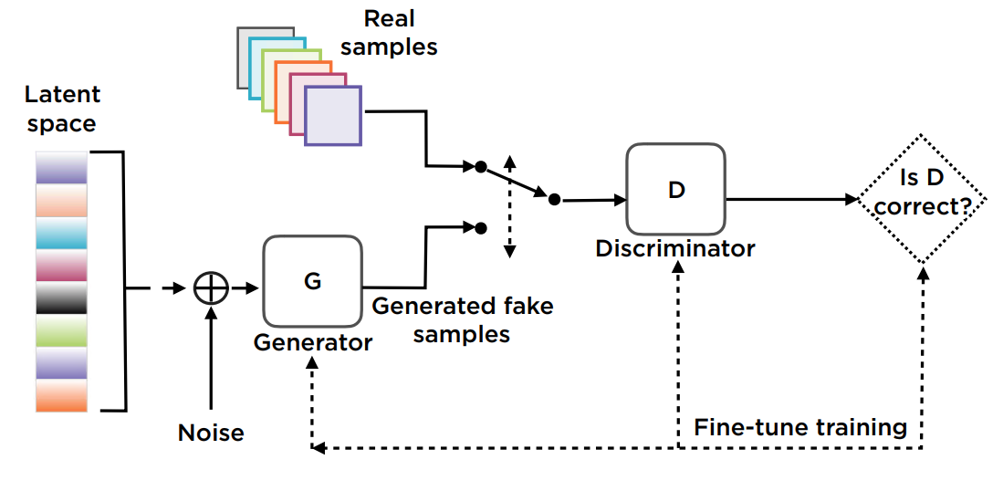
生成器
生成类似于训练数据的真实数据,以欺骗评判器。它要最大化那些被评判为真实数据的虚假数据。
评判器
生成器的输出为评判器的输入。其实就是一个真实/虚假数据的分类器。输出为两个类别的概率。它要最大化那些被评判为真实数据的真实数据,最小化那些被评判为真实数据的虚假数据。
噪声
生成随机初始数据。
Loss Function
两个网络要分别优化。采用Binary Cross-Entropy作为Loss Function。对于错误的分类,要加强惩罚。
训练过程
准备真实数据和噪声数据。
训练评判器对真实和虚假数据分类。
生成新的噪声数据。
训练生成器生成新的数据,以欺骗评判器。
使用optimizer迭代。
生成网络和评判网络互为对手。在某个时刻,生成网络能生成“真实”数据,并持续地骗过评判网络。
Leaky ReLU激活函数
为了缓解某些神经元僵死的问题,采用如下改进的ReLU激活函数: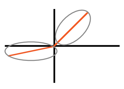
当输入大于0时,输出等于输入;当输入小于0时,输出为负值,但接近0,使用一个hyper parameter
下面使用MNIST数据集来生成虚假的手写数字。MNIST数据集的每个图像为28×28的灰度图。
生成的图像如下: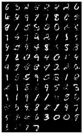
import os
import numpy as np
import torch
import torchvision
import torch.nn as nn
from torchvision import transforms
from torchvision.utils import save_image

batch_size = 100

device = torch.device('cuda' if torch.cuda.is_available() else 'cpu')

transform = transforms.Compose([
                transforms.ToTensor(),
                transforms.Normalize((0.5,), (0.5,))])

mnist = torchvision.datasets.MNIST(root='datasets/',
                                   train=True,
                                   transform=transform,
                                   download=True)

data_loader = torch.utils.data.DataLoader(dataset=mnist,
                                          batch_size=batch_size,
                                          shuffle=True
                                          )
latent_size = 64
hidden_size = 256
image_size = 28*28
num_epochs = 100

#评判网络
D = nn.Sequential(
    nn.Linear(image_size, hidden_size),
    nn.LeakyReLU(0.2),
    nn.Dropout(0.5),
    nn.Linear(hidden_size, hidden_size),
    nn.LeakyReLU(0.2),
    nn.Dropout(0.5),
    nn.Linear(hidden_size, 1),
    nn.Sigmoid())

#生成网络
G = nn.Sequential(
    nn.Linear(latent_size, hidden_size),
    nn.ReLU(),
    nn.Linear(hidden_size, hidden_size),
    nn.ReLU(),
    nn.Linear(hidden_size, image_size),
    nn.Tanh())

D = D.to(device)
G = G.to(device)

bce_loss = nn.BCELoss()

d_optimizer = torch.optim.Adam(D.parameters(), lr=0.0002)
g_optimizer = torch.optim.Adam(G.parameters(), lr=0.0002)

total_step = len(data_loader)

for epoch in range(num_epochs):

    for i, (images, _) in enumerate(data_loader):

        images = images.reshape(batch_size, -1).to(device)

        # Create the labels which are later used as input for the BCE loss
        real_labels = torch.ones(batch_size, 1).to(device)
        fake_labels = torch.zeros(batch_size, 1).to(device)

        # ================================================================== #
        #                      Train the discriminator                       #
        # ================================================================== #

        # Compute BCE_Loss using real images where BCE_Loss(x, y): - y * log(D(x)) - (1-y) * log(1 - D(x))

        outputs = D(images)

        # Second term of the loss is always zero since real_labels == 1
        # This is what causes it to minimize the loss for real images
        d_loss_real = bce_loss(outputs, real_labels)
        real_score = outputs

        # Compute BCELoss using fake images

        z = torch.randn(batch_size, latent_size).to(device)
        fake_images = G(z)

        outputs = D(fake_images)

        # First term of the loss is always zero since fake_labels == 0
        # This is what causes it to maximize the loss for fake images
        d_loss_fake = bce_loss(outputs, fake_labels)
        fake_score = outputs

        # Backprop and optimize
        d_loss = d_loss_real + d_loss_fake

        d_optimizer.zero_grad()
        g_optimizer.zero_grad()

        d_loss.backward()
        d_optimizer.step()

        # ================================================================== #
        #                        Train the generator                         #
        # ================================================================== #

        # Compute loss with fake images

        z = torch.randn(batch_size, latent_size).to(device)
        fake_images = G(z)
        outputs = D(fake_images)

        # We train G to maximize log(D(G(z)) instead of minimizing log(1-D(G(z)))
        # For the reason, see the last paragraph of section 3. https://arxiv.org/pdf/1406.2661.pdf

        g_loss = bce_loss(outputs, real_labels)

        # Backprop and optimize
        d_optimizer.zero_grad()
        g_optimizer.zero_grad()

        g_loss.backward()
        g_optimizer.step()

        if (i+1) % 200 == 0:
            print('Epoch [{}/{}], Step [{}/{}], d_loss: {:.4f}, g_loss: {:.4f}, D(x): {:.2f}, D(G(z)): {:.2f}'
                  .format(epoch, num_epochs, i+1, total_step, d_loss.item(), g_loss.item(),
                          real_score.mean().item(), fake_score.mean().item()))

    fake_images = fake_images.reshape(fake_images.size(0), 1, 28, 28)